
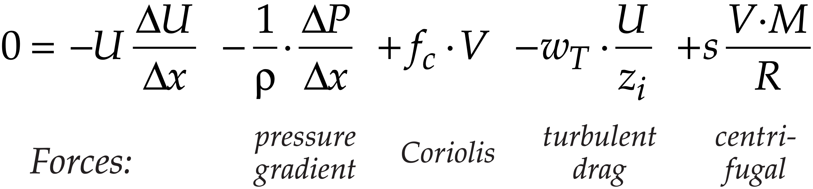
When air accelerates to create wind, forces that are a function of wind speed also change. As the winds continue to accelerate under the combined action of all the changing forces, feedbacks often occur to eventually reach a final wind where the forces balance. With a zero net force, there is zero acceleration. Such a final, equilibrium, state is called steady state: \(\ \begin \frac=0, \quad \frac=0\tag\end\) Caution: Steady state means no further change to the non-zero winds. Do not assume the winds are zero. Under certain idealized conditions, some of the forces in the equations of motion are small enough to be neglected. For these situations, theoretical steady-state winds can be found based on only the remaining larger-magnitude forces. These theoretical winds are given special names, as listed in Table 10-4. These winds are examined next in more detail. As we discuss each theoretical wind, we will learn where we can expect these in the real atmosphere.
| Table 10-4. Names of idealized steady-state horizontal winds, and the forces that govern them. | ||||
 Wind Name Wind Name | ||||
| Geostrophic | • | • | ||
| Gradient | • | • | • | |
| Atm.Bound. Layer | • | • | • | |
| ABL Gradient | • | • | • | • |
| Cyclostrophic | • | • | ||
| Inertial | • | • | ||
| Antitriptic | • | • | ||
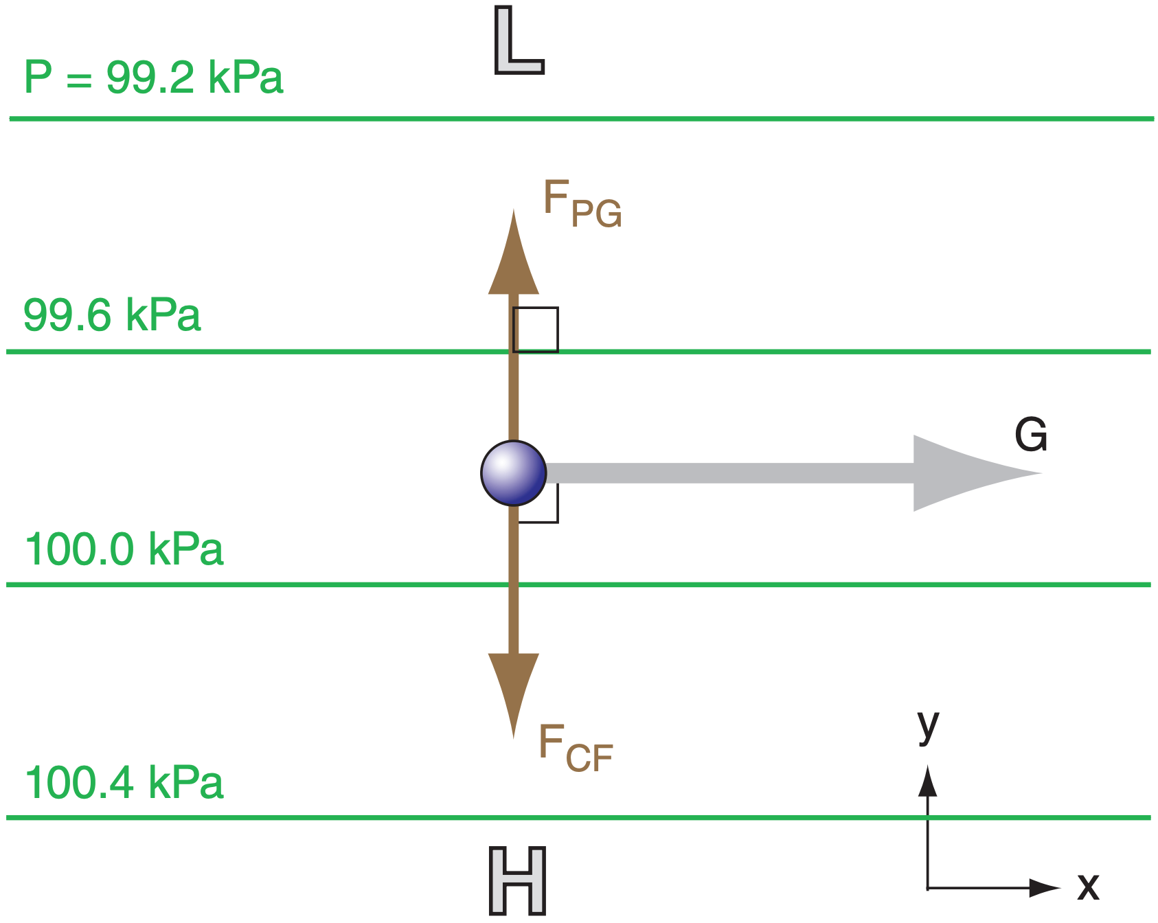
For special conditions where the only forces are Coriolis and pressure-gradient (Fig. 10.8), the resulting steady-state wind is called the geostrophic wind, with components (Ug , Vg). For this special case, the only terms remaining in, eqs. (10.23) are: \(\ \begin 0=-\frac \cdot \frac+f_ \cdot V\tag\end\) \(\ \begin 0=-\frac \cdot \frac-f_ \cdot u\tag\end\) Define U ≡ Ug and V ≡ Vg in the equations above, and then solve for these wind components: \(\ \begin U_=-\frac<\rho \cdot f_> \cdot \frac\tag\end\) \(\ \begin V_=+\frac<\rho \cdot f_> \cdot \frac\tag\end\) where fc = (1.4584x10 –4 s –1 )·sin(latitude) is the Coriolis parameter, ρ is air density, and ∆P/∆x and ∆P/∆y are the horizontal pressure gradients.
Sample Application Find geostrophic wind components at a location where ρ = 1.2 kg m –3 and fc = 1.1x10 –4 s –1 . Pressure decreases by 2 kPa for each 800 km of distance north. Find the Answer Given: fc =1.1x10 –4 s –1 , ∆P= –2 kPa, ρ=1.2 kg m –3 , ∆y=800 km. Find: (Ug , Vg) = ? m s –1 But ∆P/∆x = 0 implies Vg = 0. For Ug, use eq. (10.26a): \(U_=\frac <\left(1.2 \mathrm
 Real winds are nearly geostrophic at locations where isobars or height contours are relatively straight, for altitudes above the atmospheric boundary layer. Geostrophic winds are fast where isobars are packed closer together. The geostrophic wind direction is parallel to the height contours or isobars. In the N. (S.) hemisphere the wind direction is such that low pressure is to the wind’s left (right), see Fig. 10.9. The magnitude G of the geostrophic wind is: \(\ \begin G=\sqrt^+V_^>\tag\end\)
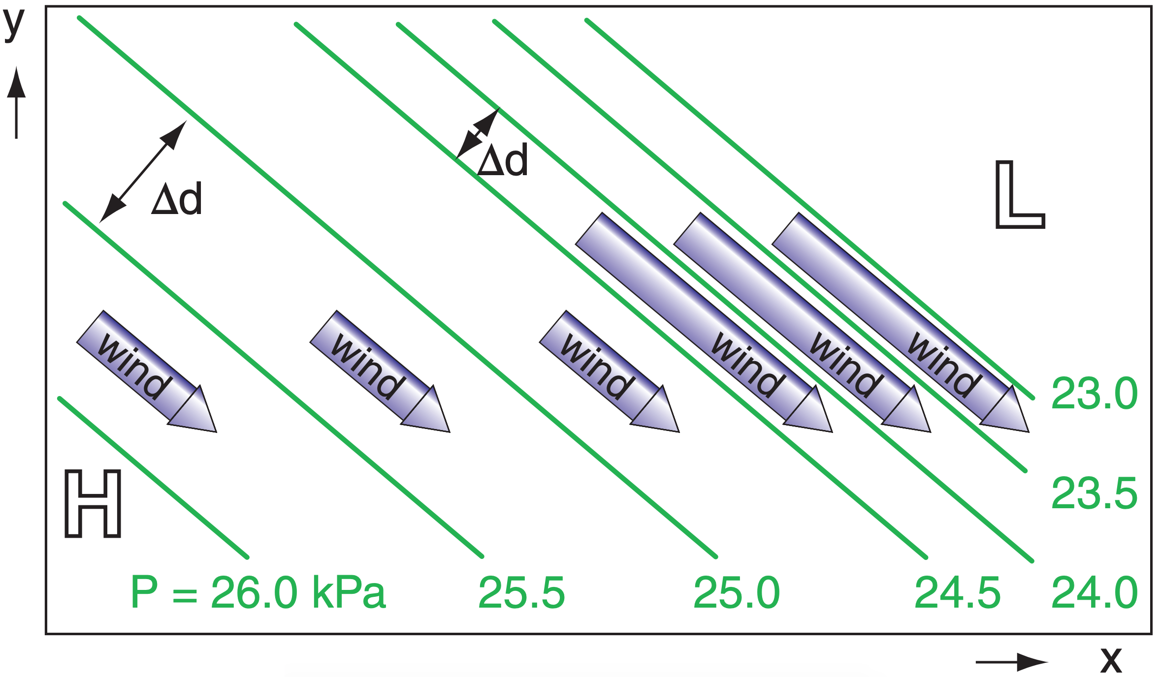
 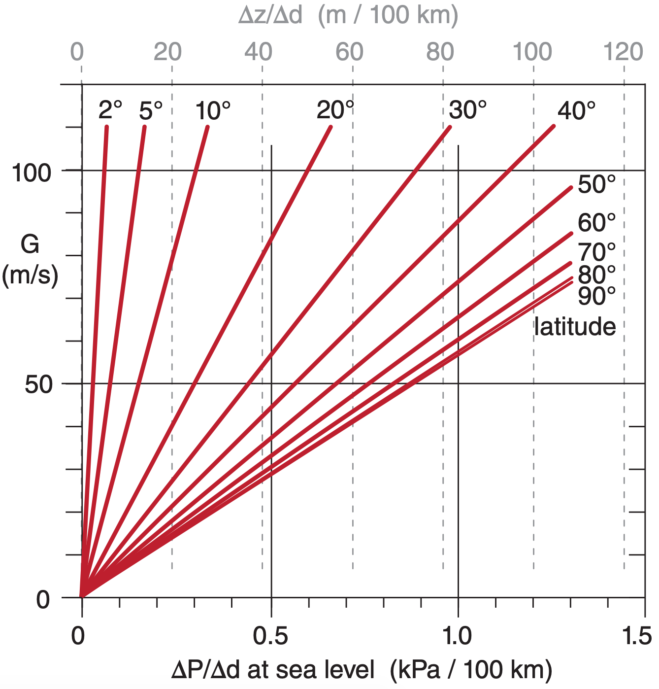 If ∆d is the distance between two isobars (in the direction of greatest pressure change; namely, perpendicular to the isobars), then the magnitude (Fig. 10.10) of the geostrophic wind is: \(\ \begin G=\left|\frac> \cdot \frac\right|\tag\end\) Above sea level, weather maps are often on isobaric surfaces (constant pressure charts), from which the geostrophic wind (Fig. 10.10) can be found from the height gradient (change of height of the isobaric surface with horizontal distance): \(\ \begin U_=-\frac<|g|>> \cdot \frac\tag\end\) \(\ \begin V_=+\frac<|g|>> \cdot \frac\tag\end\) where the Coriolis parameter is fc , and gravitational acceleration is |g| = 9.8 m·s –2 . The corresponding magnitude of geostrophic wind on an isobaric chart is: \(\ \begin G=\left|\frac> \cdot \frac\right|\tag\end\)
Sample Application Find the geostrophic wind for a height increase of 50 m per 200 km of distance toward the east. Assume, fc = 0.9x10 –4 s –1 . Find the Answer Given: ∆x = 200 km, ∆z = 50 m, fc = 0.9x10 –4 s –1 . Find: G = ? m s –1 . No north-south height gradient, thus Ug = 0. Apply eq. (10.29b) and set G = Vg : \(V_=+\frac<|g|>> \cdot \frac=\left(\frac^>^>\right) \cdot\left(\frac>>\right)=27.2 \mathrm^\) Check: Physics & units OK. Agrees with Fig. 10.10. Exposition: If height increases towards the east, then you can imagine that a ball placed on such a surface would roll downhill toward the west, but would turn to its right (toward the north) due to Coriolis force.
How does an air parcel, starting from rest, approach the final steady-state geostrophic wind speed G sketched in Fig. 10.8? Start with the equations of horizontal motion (10.23), and ignore all terms except the tendency, pressuregradient force, and Coriolis force. Use the definition of geostrophic wind (eqs. 10.26) to write the resulting simplified equations as: \(\Delta U / \Delta t=-f_
\(\Delta V / \Delta t=f_
\(V_>=V_>+\Delta t \cdot f_ 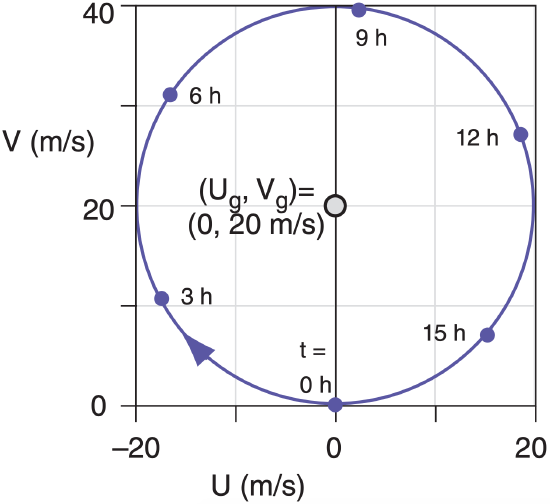 Surprisingly, the winds never reach geostrophic equilibrium, but instead rotate around the geostrophic wind. This is called an inertial oscillation, with period of 2·π/fc. For our case, the period is 17.45 h. Twice this period is called a pendulum day.
 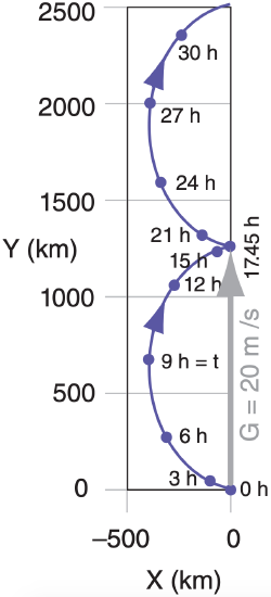 The net result in the figure below is that the wind indeed moves at the geostrophic speed of 20 m s–1 to the north (≈ 1250 km in 17.45 h), but along the way it staggers west and east with an additional ageostrophic (non-geostrophic) part. Inertial oscillations are sometimes observed at night in the atmospheric boundary layer, but rarely higher in the atmosphere. Why not? (1) The ageostrophic component of wind (wind from the East in this example) moves air mass, and changes the pressure gradient. (2) Friction damps the oscillation toward a steady wind.
If the geopotential Φ = |g|·z is substituted in eqs. (10.29), the resulting geostrophic winds are: \(\ \begin U_=-\frac> \cdot \frac\tag\end\) \(\ \begin V_=\frac> \cdot \frac\tag\end\)
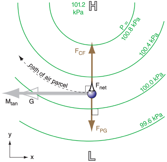
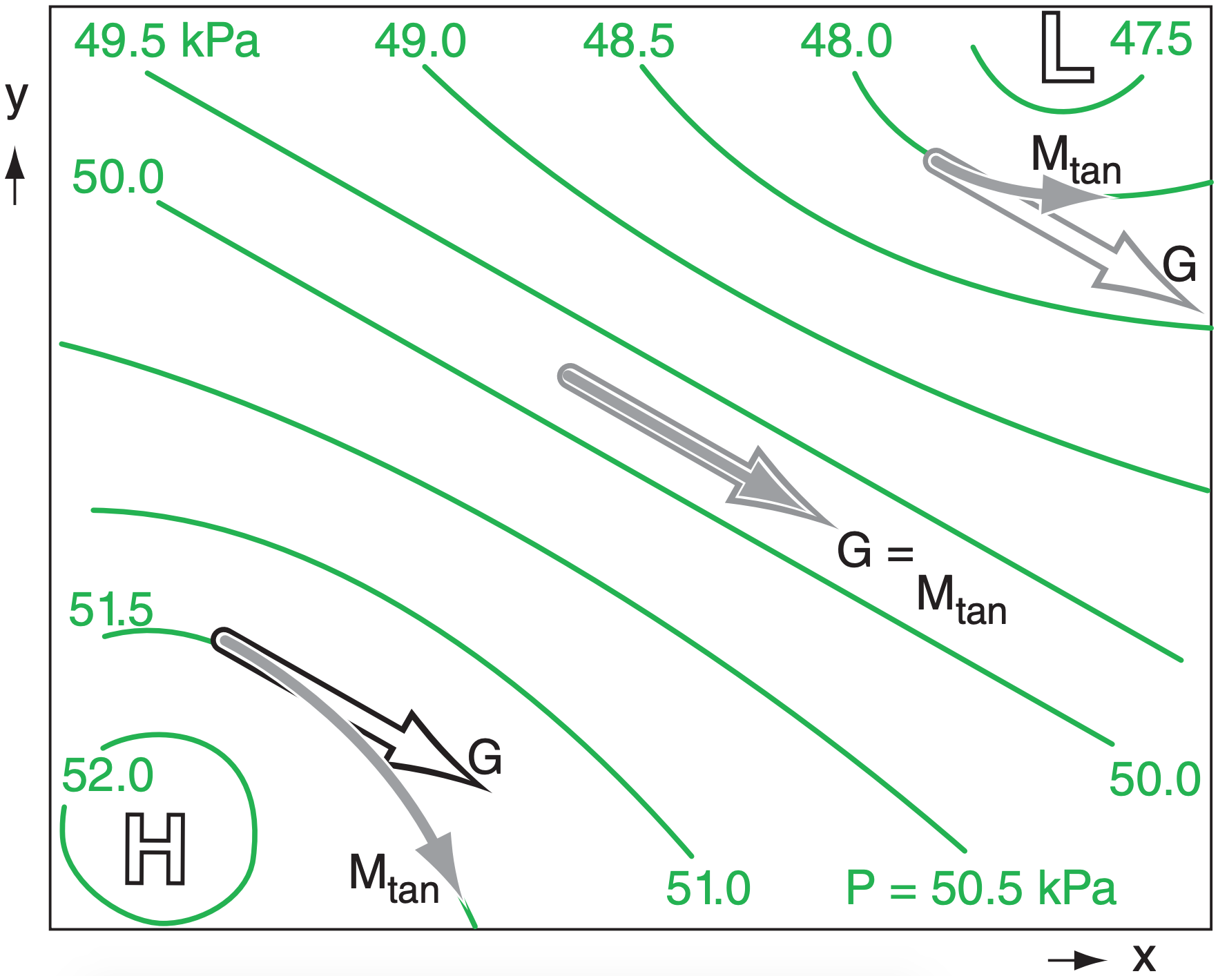
If there is no turbulent drag, then winds tend to blow parallel to isobar lines or height-contour lines even if those lines are curved. However, if the lines curve around a low-pressure center (in either hemisphere), then the wind speeds are subgeostrophic (i.e., slower than the theoretical geostrophic wind speed). For lines curving around high-pressure centers, wind speeds are supergeostrophic (faster than theoretical geostrophic winds). These theoretical winds following curved isobars or height contours are known as gradient winds. Gradient winds differ from geostrophic winds because Coriolis force FCF and pressure-gradient force FPG do not balance, resulting in a non-zero net force Fnet. This net force is called centripetal force, and is what causes the wind to continually change direction as it goes around a circle (Figs. 10.11 & 10.12). By describing this change in direction as causing an apparent force (centrifugal), we can find the equations that define a steady-state gradient wind: \(\ \begin 0=-\frac \cdot \frac+f_ \cdot V+s \cdot \frac \tag\end\) \(\ \begin 0=-\frac \cdot \frac-f_ \cdot U-s \cdot \frac\tag\end\) 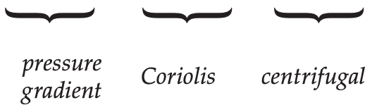 Because the gradient wind is for flow around a circle, we can frame the governing equations in radial coordinates, such as for flow around a low: \(\ \begin \frac \cdot \frac=f_ \cdot M_+\frac
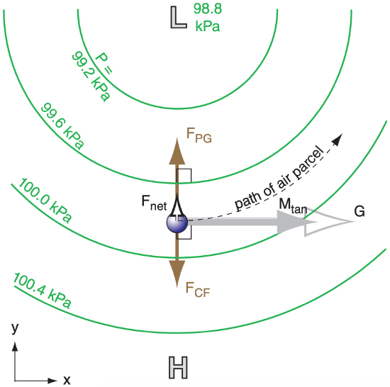
 By re-arranging eq. (10.32) and plugging in the definition for geostrophic wind speed G, you can get an implicit solution for the gradient wind Mtan: \(\ \begin M_<\mathrm
Sample Application What radius of curvature causes the gradient wind to equal the geostrophic wind? Find the Answer Given: Mtan = G Find: R = ? km Use eq. (10.33), with Mtan = G: G = G ± G 2 /( fc·R) This is a valid equality G = G only when the last term in eq. (10.33) approaches zero; i.e., in the limit of R = ∞ . Check: Eq. (10.33) still balances in this limit. Exposition: Infinite radius of curvature is a straight line, which (in the absence of any other forces such as turbulent drag) is the condition for geostrophic wind.
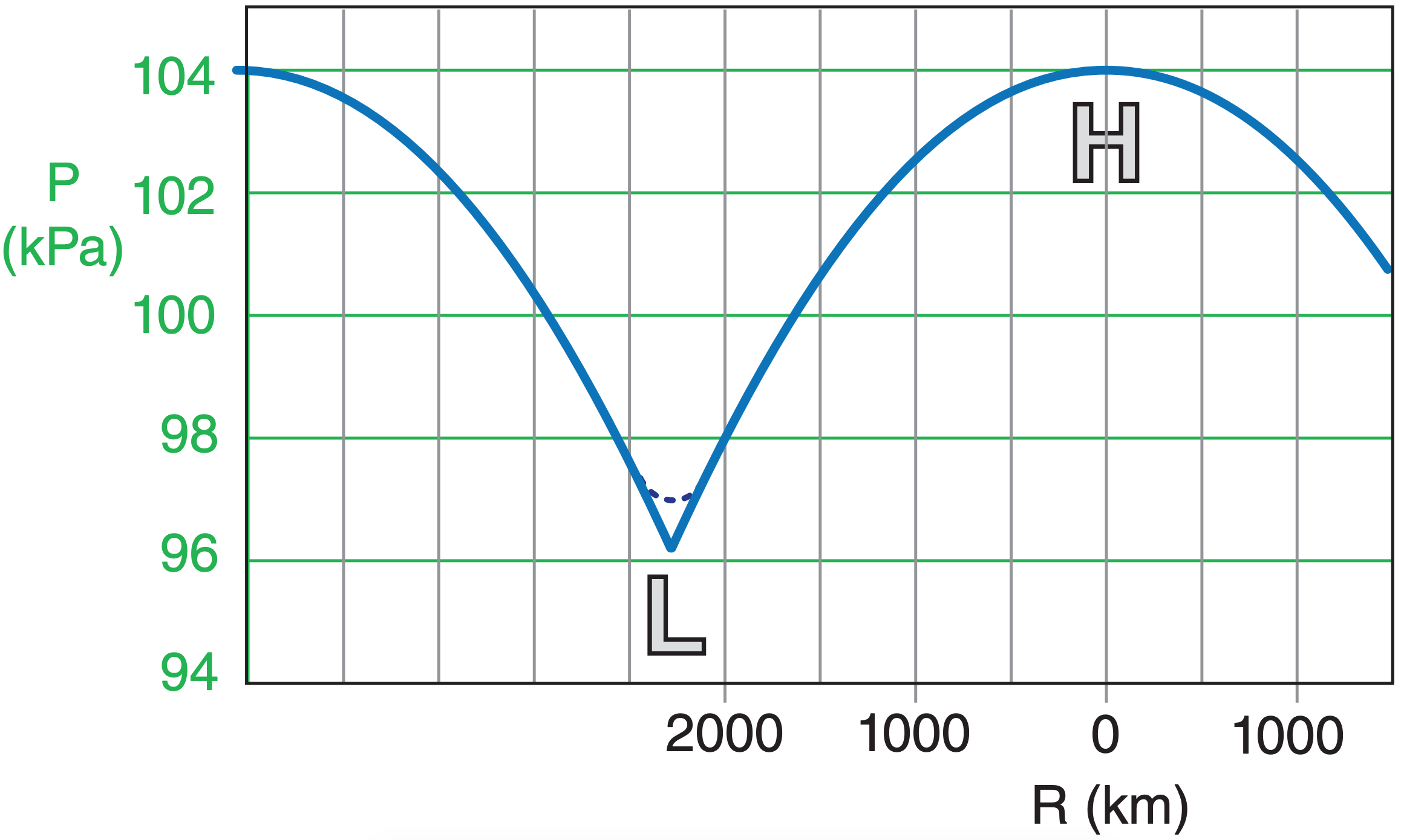
The Rossby number (Ro) is a dimensionless ratio defined by \(R o=\frac \cdot L> \quad\) or \(\quad R o=\frac \cdot R>\) where M is wind speed, fc is the Coriolis parameter, L is a characteristic length scale, and R is radius of curvature. In the equations of motion, suppose that advection terms such as U·∆U/∆x are order of magnitude M 2 /L, and Coriolis terms are of order fc·M. Then the Rossby number is like the ratio of advection to Coriolis terms: (M 2 /L) / (fc·M) = M/(fc·L) = Ro. Or, we could consider the Rossby number as the ratio of centrifugal (order of M 2 /R) to Coriolis terms, yielding M/(fc·R) = Ro. Use the Rossby number as follows. If Ro < 1, then Coriolis force is a dominant force, and the flow tends to become geostrophic (or gradient, for curved flow). If Ro >1, then the flow tends not to be geostrophic. For example, a midlatitude cyclone (low-pressure system) has approximately M = 10 m s –1 , fc = 10 –4 s –1 , and R = 1000 km, which gives Ro = 0.1 . Hence, midlatitude cyclones tend to adjust toward geostrophic balance, because Ro < 1. In contrast, a tornado has roughly M = 50 m s –1 , fc = 10 –4 s –1 , and R = 50 m, which gives Ro = 10,000, which is so much greater than one that geostrophic balance is not relevant.
 Eq. (10.33) is a quadratic equation that has two solutions. One solution is for the gradient wind Mtan around a cyclone (i.e., a low): \(\ \begin M_<\mathrm
Sample Application If G = 10 m s –1 , find the gradient wind speed & Roc, given fc = 10 –4 s –1 and a radius of curvature of 500 km? Find the Answer Given: G = 10 m s –1 , R = 500 km, fc = 10 –4 s –1 Find: Mtan = ? m s –1 , Roc = ? (dimensionless) Use eq. (10.34a): Mtan = 0.5 · (10 -4 s -1 ) ·(500000m)· \([-1+\sqrt <\left(10^<-4>s^\right) \cdot(500000 m)>>]=\underline<8.54 m s^>\) Use eq. (10.35): \(R o_=\frac <(10 \mathrm/ \mathrm)> <\left(10^<-4>\mathrm^\right) \cdot\left(5 \times 10^ \mathrm\right)>=\underline\) Check: Physics & units are reasonable. Exposition: The gradient wind is slower than geostrophic and is in geostrophic balance.
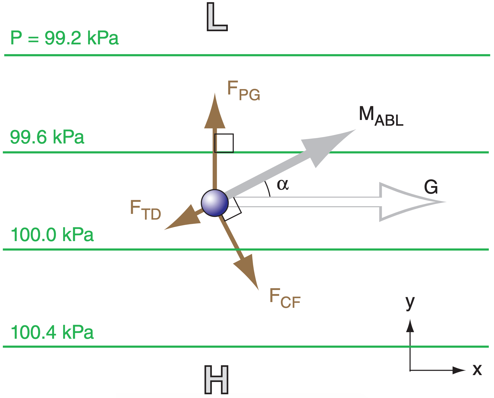
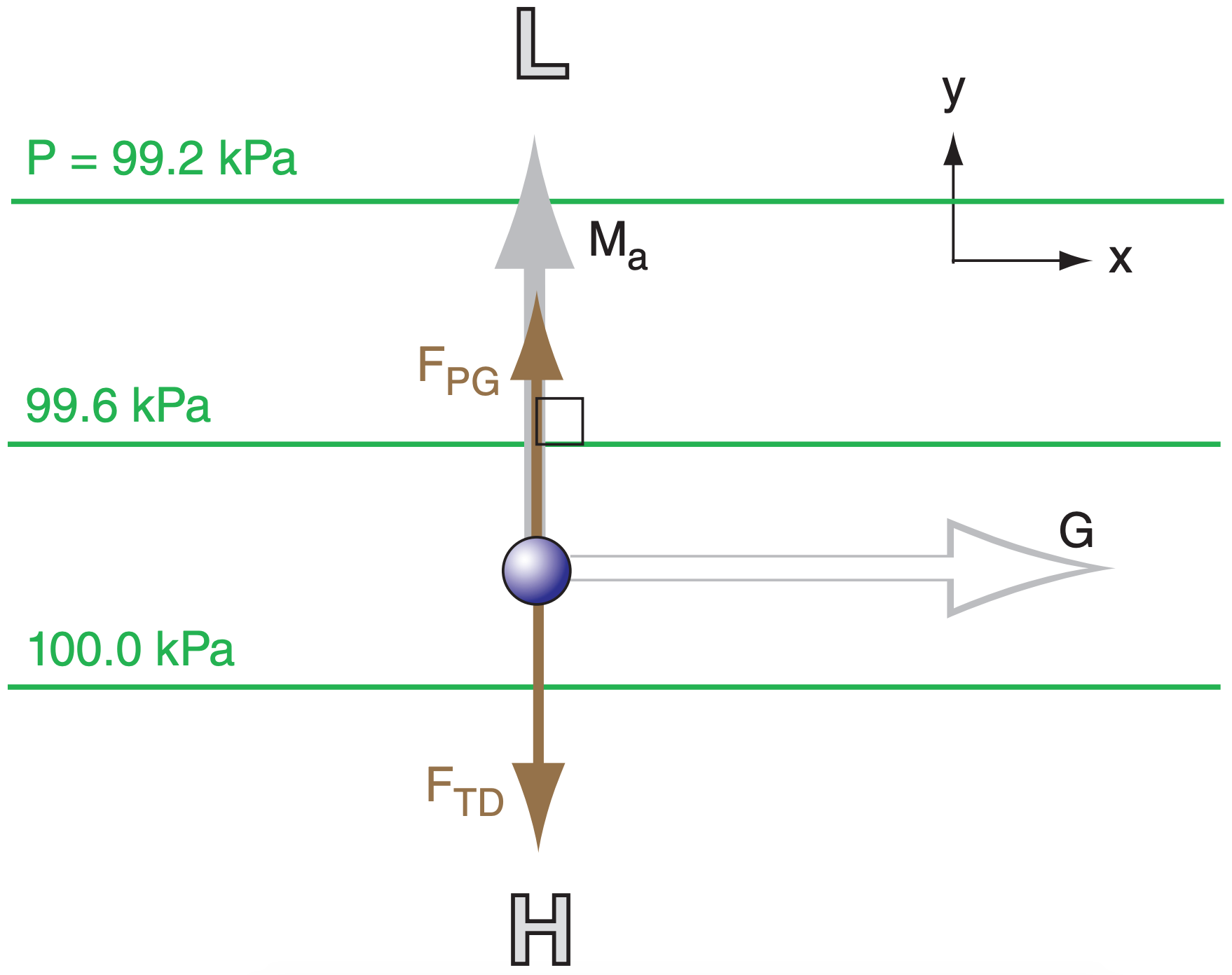
If you add turbulent drag to winds that would have been geostrophic, the result is a subgeostrophic (slower-than-geostrophic) wind that crosses the isobars at angle (α) (Fig. 10.17). This condition is found in the atmospheric boundary layer (ABL) where the isobars are straight. The force balance at steady state is: \(\ \begin 0=-\frac \cdot \frac+f_ \cdot V-w_ \cdot \frac>\tag\end\) \(\ \begin 0=-\frac \cdot \frac-f_ \cdot U-w_ \cdot \frac>\tag\end\) Namely, the only forces acting for this special case are pressure gradient, Coriolis, and turbulent drag (Fig. 10.17). Replace U with UABL and V with VABL to indicate these winds are in the ABL. Eqs. (10.38) can be rearranged to solve for the ABL winds, but this solution is implicit (depends on itself): \(\ \begin U_=U_-\frac
Sample Application For statically neutral conditions, find the winds in the boundary layer given: zi = 1.5 km, Ug = 15 m s –1 , Vg = 0, fc = 10 –4 s –1 , and CD = 0.003. What is the crossisobar wind angle? Find the Answer Given: zi = 1.5 km, Ug = 15 m s –1 , Vg = 0, fc = 10 –4 s –1 , CD = 0.003. Find: VABL =? m s –1 , UABL =? m s –1 , MABL =? m s –1 , α = ? ° First: G =(Ug 2 + Vg 2 ) 1/2 = 15 m s –1 . Now apply eq.(10.41) \(a=\frac <\left(10^<-4>\mathrm^\right) \cdot(1500 \mathrm)>=0.02 \mathrm / \mathrm\) Check: a·G = (0.02 s m –1 )·(15 m s –1 ) =0.3 (is < 1. Good.) UABL=[1–0.35·(0.02s m –1 )·(15m s –1 )]·(15m s –1 )≈13.4m s –1 VABL=[1–0.5·(0.02s m –1 )·(15m s –1 )]· (0.02s m –1 )·(15m s –1 )·(15m s –1 ) ≈ 3.8 m s –1 \(M_=\sqrt
Sample Application For statically unstable conditions, find winds in the ABL given Vg = 0, Ug = 5 m s –1 , wB = 50 m s –1 , zi = 1.5 km, bD = 1.83x10 –3 , and fc = 10 –4 s –1 . What is the crossisobar wind angle? Find the Answer Given: (use convective boundary layer values above) Find: MABL =? m s –1 , VABL =? m s –1 , UABL =? m s –1 , α =?° Apply eqs. (10.42): \(c_=\frac<\left(1.83 \times 10^<-3>\right) \cdot(50 \mathrm / \mathrm)> <\left(10^<-4>\mathrm^\right) \cdot(1500 \mathrm)>=0.61(\) dimensionless) c2 = 1/[1+(0.61) 2 ] = 0.729 (dimensionless) UABL = 0.729·[(5m s –1 ) – 0 ] = 3.6 m s –1 VABL = 0.729·[0 + (0.61)·(5m s –1 )] = 2.2 m s –1 Use eq. (10.40): MABL = [U 2 ABL + V 2 ABL ] 1/2 = 4.2 m s –1 α =tan –1 (VABL/UABL) = tan –1 (2.2/3.6) = 31.4° Check: Physics & units are reasonable. Exposition: Again, drag slows the wind and causes it to cross the isobars toward low pressure. The ABL wind direction is 238.6°.
For curved isobars in the atmospheric boundary layer (ABL), there is an imbalance of the following forces: Coriolis, pressure-gradient, and drag. This imbalance is a centripetal force that makes ABL air spiral outward from highs and inward toward lows (Fig. 10.18). An example was shown in Fig. 10.1. 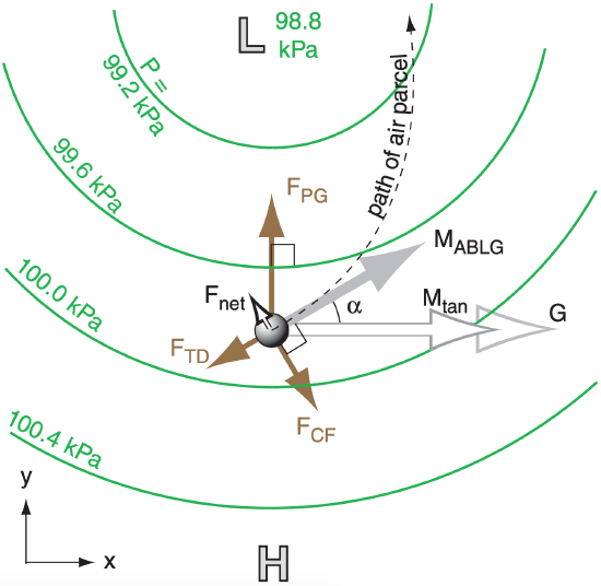 If we devise a centrifugal force equal in magnitude but opposite in direction to the centripetal force, then the equations of motion can be written for spiraling flow that is steady over any point on the Earth’s surface (i.e., NOT following the parcel): \(\ \begin 0=-\frac \cdot \frac+f_ \cdot V-w_ \cdot \frac>+s \cdot \frac\tag\end\) \(\ \begin 0=-\frac \cdot \frac-f_ \cdot u-w_ \cdot \frac>-s \cdot \frac\tag\end\)
 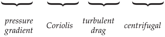 We can anticipate that the ABLG winds should be slower than the corresponding gradient winds, and should cross isobars toward lower pressure at some small angle α (see Fig. 10.19).
 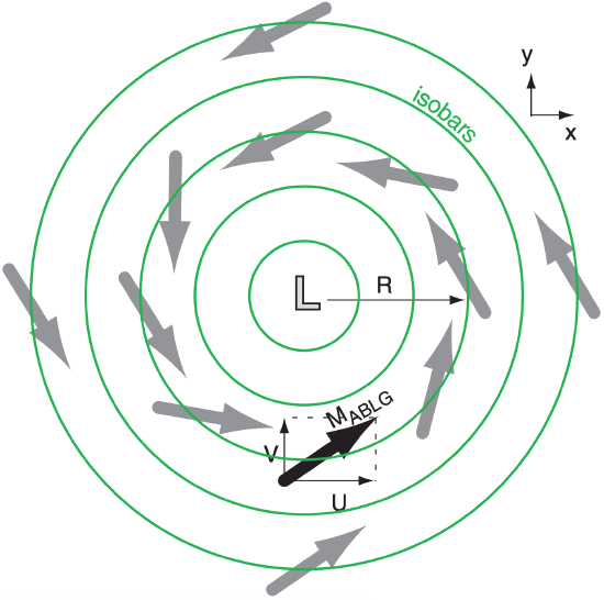 Lows are often overcast and windy, implying that the atmospheric boundary layer is statically neutral. For this situation, the transport velocity is given by: \(\ \begin w_<\mathrm>=C_ \cdot M=C_ \cdot \sqrt+V^>\tag\end\) Because this parameterization is nonlinear, it increases the nonlinearity (and the difficulty to solve), eqs. (10.43). Highs often have mostly clear skies with light winds, implying that the atmospheric boundary layer is statically unstable during sunny days, and statically stable at night. For daytime, the transport velocity is given by: \(\ \begin w_=b_ \cdot w_\tag\end\) This parameterization for wB is simple, and does not depend on wind speed. For statically stable conditions during fair-weather nighttime, steady state is unlikely, meaning that eqs. (10.43) do not apply. Nonlinear coupled equations (10.43) are difficult to solve analytically. However, we can rewrite the equations in a way that allows us to iterate numerically toward the answer (see the INFO box below for instructions). The trick is to not assume steady state. Namely, put the tendency terms (∆U/∆t , ∆V/∆t) back in the left hand sides (LHS) of eqs. (10.43). But recall that ∆U/∆t = [U(t+∆t) – U]/∆t, and similar for V. For this iterative approach, first re-frame eqs. (10.43) in cylindrical coordinates, where (U, V) are the (tangential, radial) components, respectively (see Fig. 10.19). Also, use G, the geostrophic wind definition of eq. (10.28), to quantify the pressure gradient. For a cyclone in the Northern Hemisphere (for which s = +1 from Table 10-2), the atmospheric boundary layer gradient wind eqs. (10.43) become: \(\ \begin M=\left(U^+V^\right)^\tag\end\) \(\ \begin U(t+\Delta t)=U+\Delta t \cdot\left[f_ \cdot V-\frac
Sample Application If G = 10 m s –1 at R = 400 km from the center of a N. Hem. cyclone, CD = 0.02, zi = 1 km, and fc = 10 –4 s –1 , then find the ABLG wind speed and components. Find the Answer Given: (see the data above) Find: MBLG = ? m s –1 , UBLG = ? m s –1 , VBLG = ? m s –1 , Use a spreadsheet to iterate (as discussed in the INFO box) eqs. (10.44) & (1.1) with a time step of ∆t = 1200 s. Use U = V = 0 as a first guess.
| G (m/s)= | 10 | zi (km)= | 1 | ||
| R (km)= | 400 | fc (s –1 )= | 0.0001 | ||
| CD = | 0.02 | ∆t(s)= | 1200 | ||
| Iteration | UABLG | VABLG | MABLG | ∆UABLG | ∆ VABLG |
| Counter | (m s –1 ) | (m s –1 ) | (m s –1 ) | (m s –1 ) | (m s –1 ) |
| 0 | 0.00 | 0.00 | 0.00 | 0.000 | 1.200 |
| 1 | 0.00 | 1.20 | 1.20 | 0.148 | 1.165 |
| 2 | 0.15 | 2.37 | 2.37 | 0.292 | 1.047 |
| 3 | 0.44 | 3.41 | 3.44 | 0.408 | 0.861 |
| 4 | 0.85 | 4.27 | 4.36 | 0.480 | 0.640 |
| 5 | 1.33 | 4.91 | 5.09 | 0.502 | 0.420 |
| . . . | |||||
| 29 | 4.16 | 4.33 | 6.01 | -0.003 | 0.001 |
| 30 | 4.16 | 4.33 | 6.01 | -0.002 | 0.001 |
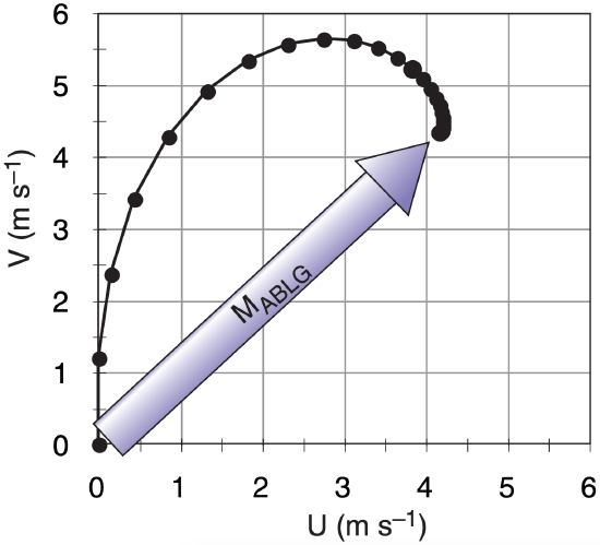
The evolution of the iterative solution is plotted at right as it approaches the final answer of UABLG = 4.16 m s –1 , VABLG = 4.33 m s –1 , MABLG= 6.01 m s –1 , where (UABLG , VABLG) are (tangential, radial) parts. Check: Physics & units are reasonable. You should do the following “what if” experiments on the spreadsheet to check the validity. I ran experiments using a modified spreadsheet that relaxed the results using a weighted average of new and previous winds. (a) As R approaches infinity and CD approaches zero, then MABLG should approach the geostrophic wind G. I got UABLG = G = 10 m s –1 , VABLG = 0. (b) For finite R and 0 drag, then MABLG should equal the gradient wind Mtan. I got UABLG = 8.28 m s –1 , VABLG = 0. (c) For finite drag but infinite R, then MABLG should equal the atmospheric boundary layer wind MABL. I got UABLG = 3.91 m s –1 , VABLG = 4.87 m s –1 . Because this ABL solution is based on the full equations, it gives a better answer than eqs. (10.41). Exposition: If you take slightly larger time steps, the solution converges faster. But if ∆t is too large, the iteration method fails (i.e., blows up).
(1) Make an initial guess for (U, V), such as (0, 0). (2) Use these (U, V) values in the right sides of eqs. (10.44) and (1.1), and solve for the new values of [U(t+∆t), V(t+∆t)]. (3) In preparation for the next iteration, let U = U(t+∆t) , and V = V(t+∆t) . (4) Repeat steps 2 and 3 using the new (U, V) on the right hand sides . (5) Keep iterating. Eventually, the [U(t+∆t), V(t+∆t)] values stop changing (i.e., reach steady state), giving UABLG = U(t+∆t), and VABLG = V(t+∆t). Because of the repeated, tedious calculations, I recommend you use a spreadsheet (see the Sample Application) or write your own computer program. As you can see from the Sample Application, the solution spirals toward the final answer as a damped inertial oscillation.
For daytime fair weather conditions in anticyclones, you could derive alternatives to eqs. (10.44) that use convective parameterizations for atmospheric boundary layer drag. Because eqs. (10.44) include the tendency terms, you can also use them for non-steady-state (time varying) flow. One such case is nighttime during fair weather (anticyclonic) conditions. Near sunset, when vigorous convective turbulence dies, the drag coefficient suddenly decreases, allowing the wind to accelerate toward its geostrophic equilibrium value. However, Coriolis force causes the winds to turn away from that steady-state value, and forces the winds into an inertial oscillation. See a previous INFO box titled Approach to Geostrophy for an example of undamped inertial oscillations. During a portion of this oscillation the winds can become faster than geostrophic (supergeostrophic), leading to a low-altitude phenomenon called the nocturnal jet. See the Atmospheric Boundary Layer chapter for details.
Winds in tornadoes are about 100 m s –1 , and in waterspouts are about 50 m s –1 . As a tornado first forms and tangential winds increase, centrifugal force increases much more rapidly than Coriolis force. Centrifugal force quickly becomes the dominant force that balances pressure-gradient force (Fig. 10.20). Thus, a steady-state rotating wind is reached at much slower speeds than the gradient wind speed. 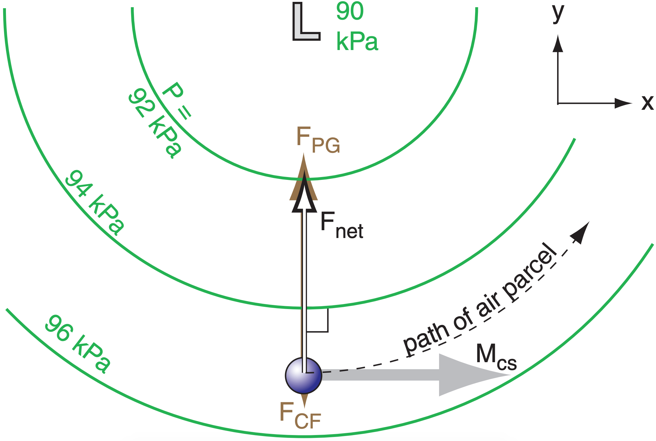 If the tangential velocity around the vortex is steady, then the steady-state force balance is: \(\ \begin 0=-\frac \cdot \frac+s \cdot \frac\tag\end\) \(\ \begin 0=-\frac \cdot \frac-s \cdot \frac\tag\end\)
  You can use cylindrical coordinates to simplify solution for the cyclostrophic (tangential) winds Mcs around the vortex. The result is: \(\ \begin M_=\sqrt<\frac \cdot \frac>\tag\end\) where the velocity Mcs is at distance R from the vortex center, and the radial pressure gradient in the vortex is ∆P/∆R. Recall from the Gradient Wind section that anticyclones cannot have strong pressure gradients, hence winds around highs are too slow to be cyclostrophic. Around cyclones (lows), cyclostrophic winds can turn either counterclockwise or clockwise in either hemisphere, because Coriolis force is not a factor.
Sample Application A 10 m radius waterspout has a tangential velocity of 45 m s –1 . What is the radial pressure gradient? Find the Answer Given: Mcs = 45 m s –1 , R = 10 m. Find: ∆P/∆R = ? kPa m –1 . Assume cyclostrophic wind, and ρ = 1 kg m –3 . Rearrange eq. (10.46): \(\frac=\frac \cdot M_^=\frac <\left(1 \mathrm
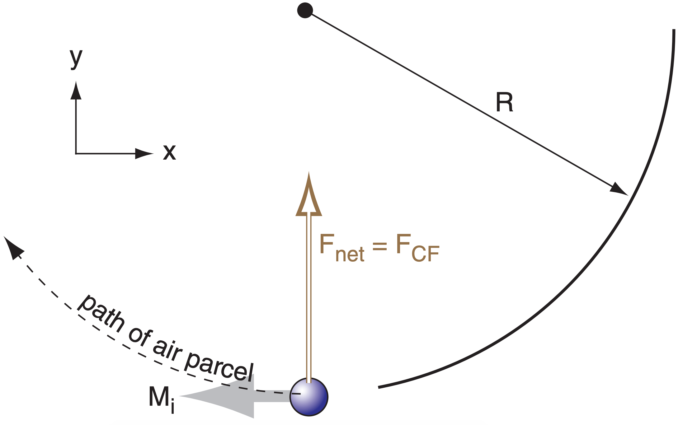
Steady-state inertial motion results from a balance of Coriolis and centrifugal forces in the absence of any pressure gradient: \(\ \begin 0=f_ \cdot M_+\frac
Sample Application For an inertial ocean current of 5 m s –1 , find the radius of curvature and time period to complete one circuit. Assume a latitude where fc = 10 –4 s –1 . Find the Answer Given: Mi = 5 m s –1 , fc = 10 –4 s –1 . Find: R = ? km, Period = ? h Use eq. (10.48): R = –(5 m s –1 ) / (10 –4 s –1 ) = –50 km Use Period = 2π/fc = 62832 s = 17.45 h Check: Units & magnitudes are reasonable. Exposition: The tracks of drifting buoys in the ocean are often cycloidal, which is the superposition of a circular inertial oscillation and a mean current that gradually translates (moves) the whole circle.
A steady-state antitriptic wind Ma could result from a balance of pressure-gradient force and turbulent drag: \(\ \begin
Sample Application In a 1 km thick convective boundary layer at a location where fc = 10 –4 s –1 , the geostrophic wind is 5 m s –1 . The turbulent transport velocity is 0.02 m s –1 . Find the antitriptic wind speed. Find the Answer Given: G = 5 m s –1 , zi = 1000 m, fc = 10 –4 s –1 , wT = 0.02 m s –1 Find: Ma = ? m s –1 Use eq. (10.50): Ma = (1000m)·(10 –4 s –1 )·(5m s –1 ) / (0.02 m s –1 ) = 25 m s –1 Check: Magnitude is too large. Units reasonable. Exposition: Eq. (10.50) can give winds of Ma > G for many convective conditions, for which case Coriolis force would be expected to be large enough that it should not be neglected. Thus, antitriptic winds are unphysical. However, for forced-convective boundary layers where drag is proportional to wind speed squared, reasonable solutions are possible.
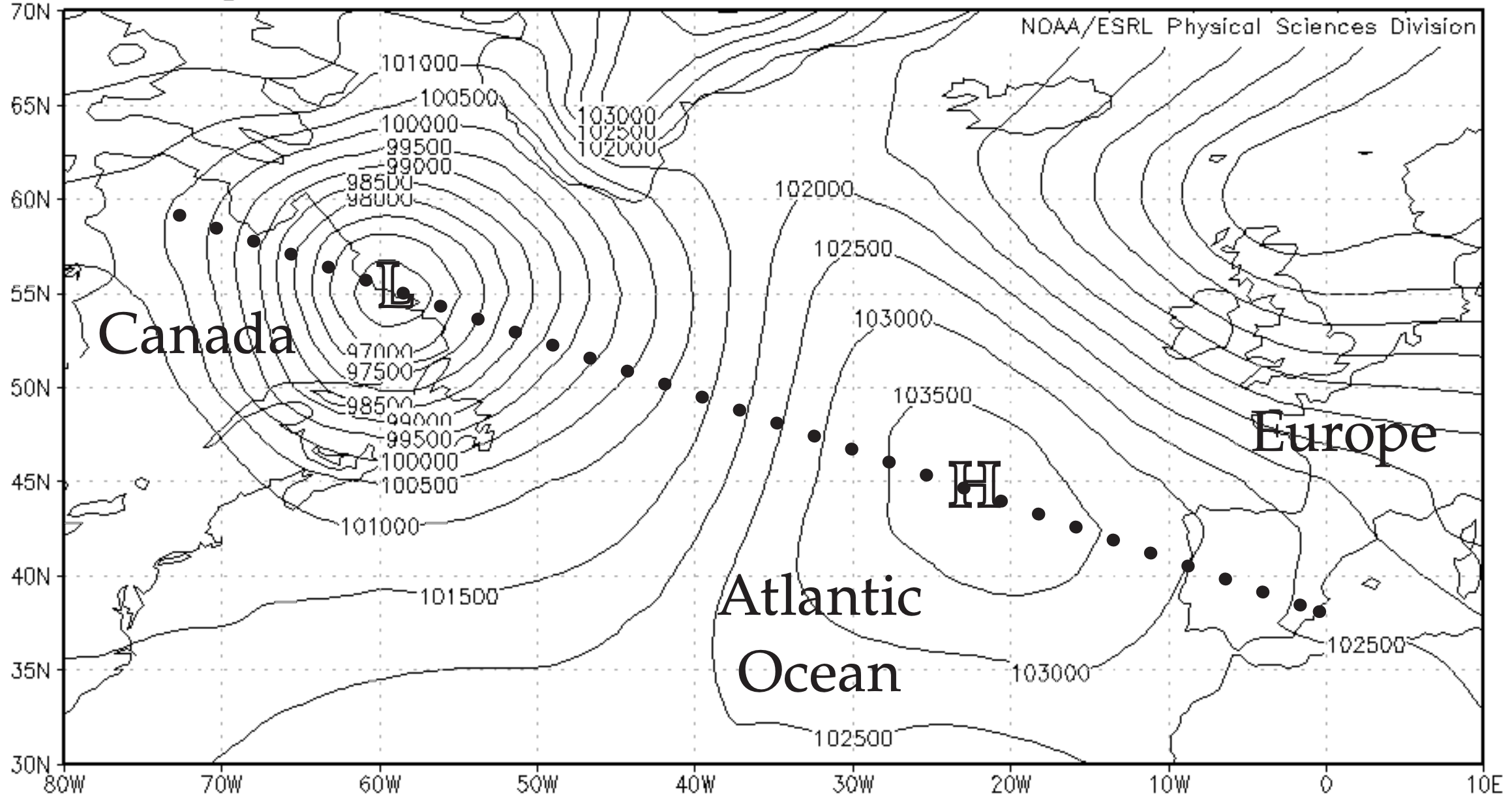
Table 10-5 summarizes the idealized horizontal winds that were discussed earlier in this chapter. On real weather maps such as Fig. 10.23, isobars or height contours have complex shapes. In some regions the height contours are straight (suggesting that actual winds should nearly equal geostrophic or boundary-layer winds), while in other regions the height contours are curved (suggesting gradient or boundary-layer gradient winds). Also, as air parcels move between straight and curved regions, they are sometimes not quite in equilibrium. Nonetheless, when studying weather maps you can quickly estimate the winds using the summary table.
| Table 10-5. Summary of horizontal winds**. | |||||
| Item | Name of Wind | Forces | Direction | Magnitude | Where Observed |
|---|---|---|---|---|---|
| 1 | geostrophic | pressure-gradient, Coriolis | parallel to straight isobars with Low pressure to the wind’s left* | faster where isobars are closer together. \(G=\left|\frac> \cdot \frac\right|\) | aloft in regions where isobars are nearly straight |
| 2 | gradient | pressure-gradient, Coriolis, centrifugal | similar to geostrophic wind, but following curved isobars. Clockwise* around Highs, counterclockwise* around Lows. | slower than geostrophic around Lows, faster than geostrophic around Highs | aloft in regions where isobars are curved |
| 3 | atmospheric boundary layer | pressure-gradient, Coriolis, drag | similar to geostrophic wind, but crosses isobars at small angle toward Low pressure | slower than geostrophic (i.e., subgeostrophic) | near the ground in regions where isobars are nearly straight |
| 4 | atmospheric boundarylayer gradient | pressure-gradient, Coriolis, drag, centrifugal | similar to gradient wind, but crosses isobars at small angle toward Low pressure | slower than gradient wind speed | near the ground in regions where isobars are curved |
| 5 | pressure-gradient, centrifugal | pressure-gradient, centrifugal | either clockwise or counterclockwise around strong vortices of small diameter | stronger for lower pressure in the vortex center | tornadoes, waterspouts (& sometimes in the eye-wall of hurricanes) |
| 6 | inertial | Coriolis, centrifugal | anticyclonic circular rotation | coasts at constant speed equal to its initial speed | ocean-surface currents |
* For Northern Hemisphere. Direction is opposite in Southern Hemisphere. ** Antitriptic winds are unphysical; not listed here.
This page titled 10.5: Horizontal Winds is shared under a CC BY-NC-SA 4.0 license and was authored, remixed, and/or curated by Roland Stull via source content that was edited to the style and standards of the LibreTexts platform.